PYL fev 2011
test of flow arround an airfoil for several angles of attack
The analytical solution are found on
Aerodynamics course
of Geordie McBain, read this and in
"Darrozès J.S.
François C. Mécanique des Fluides Incompressibles, Springer 82".
The idea of direct solution with full Laplacians is taken from freefem++ manual, read this page for the theory (explanation of the decomposition and reconstruction with the approximation of the Kutta condition).
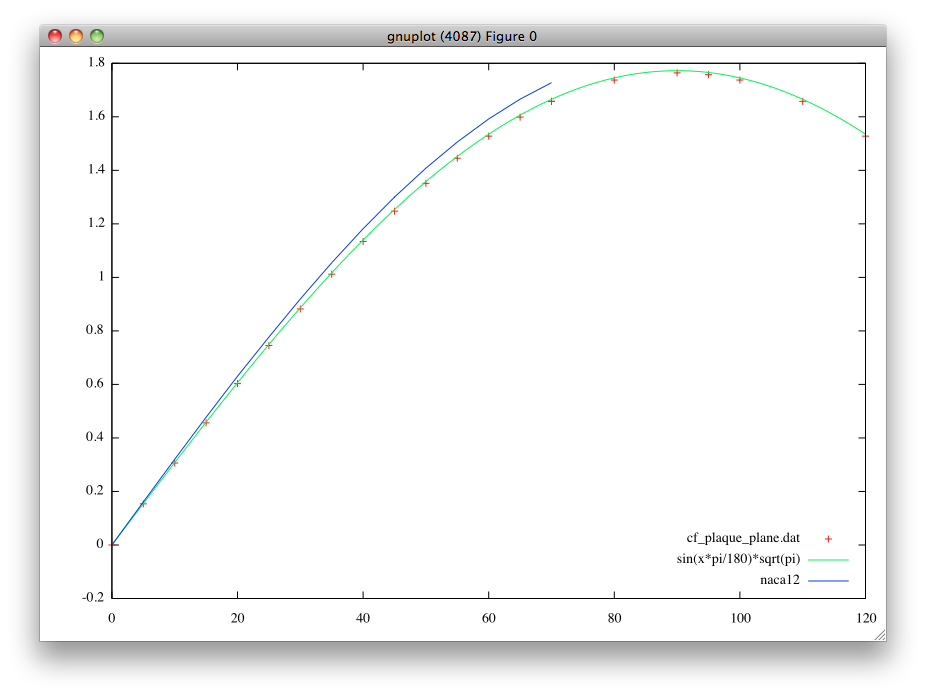
The associated freefem++ script allows to plot the following comparisons.
The "mathematica" label on the plots corresponds to the use of the following nice
Mathematica script
Application with gerris:
The wing is defined in ail.sh
with a awk script:
print x,e*(0.17735*sqrt(x)-0.075597*x - 0.212836*(x*x)+0.17363*(x*x*x)-0.06254*(x*x*x*x))
then using shapes the gts file is constructed
shapes aile.dat > aile.gts
We solve the Poisson problem for the flow arround the airfoil, for the variable P, which is in fact the stream function ψ.
∂2ψ/ ∂x2 +∂2ψ/ ∂y2 =0
so notice "
GfsPoisson" at the first line of the files
wing0.gfs and wing1.gfs.
First the problem with no circulation is solved (wing0.gfs):
far away from the wing (here a NACA0012)
∂ ψ/ ∂y= cos(α) and
∂ ψ/ ∂x= -sin(α)
so that ψ= y cos(α) - x sin(α)
at the border of the flow (the wing is of length 1, the domain of length L0) a constant velocity is imposed
for example left:
BcDirichlet P y*cos(alph*pis180)+L0/2*sin(alph*pis180)
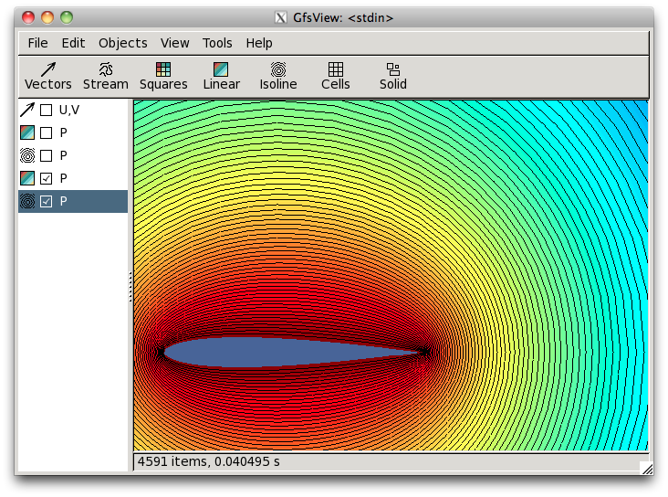
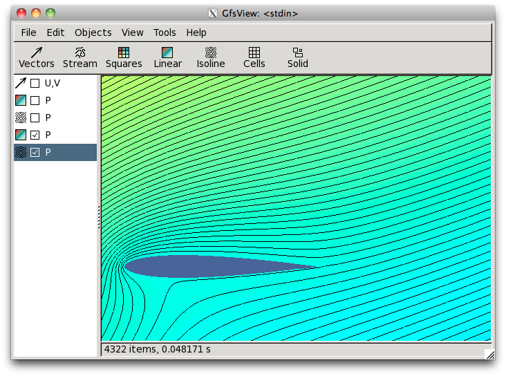
Then the problem with circulation is solved (wing1.gfs), notice that P is 0 at the border.
Then
the linear combination is taken in order to fullfit the Kutta condition.
This is done in tuning the value of the circulation. This tuning is done in writing that in the vicinity of the trailing edge the velocity u is continuous (u=∂ ψ/ ∂y is obtained by taking an approximation of ∂P/∂y)
To do that the leading edge position has been identified in ail.sh by bdf.dat and the nearby points
bdfp.dat and bdfm.dat. The P field is saved at those points
in
wing0.gfs
OutputLocation { istep = 1 } vbdfp0.dat bdfp.dat
OutputLocation { istep = 1 } vbdfm0.dat bdfm.dat
in wing1.gfs
OutputLocation { istep = 1 } vbdfp1.dat bdfp.dat
OutputLocation { istep = 1 } vbdfm1.dat bdfm.dat
and the values are extracted:
Pp0=`awk '{ print $5}' vbdfp0.dat | tail -n 1`
Pm0=`awk '{ print $5}' vbdfm0.dat | tail -n 1`
Pp1=`awk '{ print $5}' vbdfp1.dat | tail -n 1`
Pm1=`awk '{ print $5}' vbdfm1.dat | tail -n 1`
and the proper circulation
gamma=$(awk "BEGIN{ print -($Pp0+$Pm0)/($Pp1+$Pm1-2.0)}")
the final computation uses this value.
example of run
./ail.sh 10 -s
gives first the problem with no circulation,
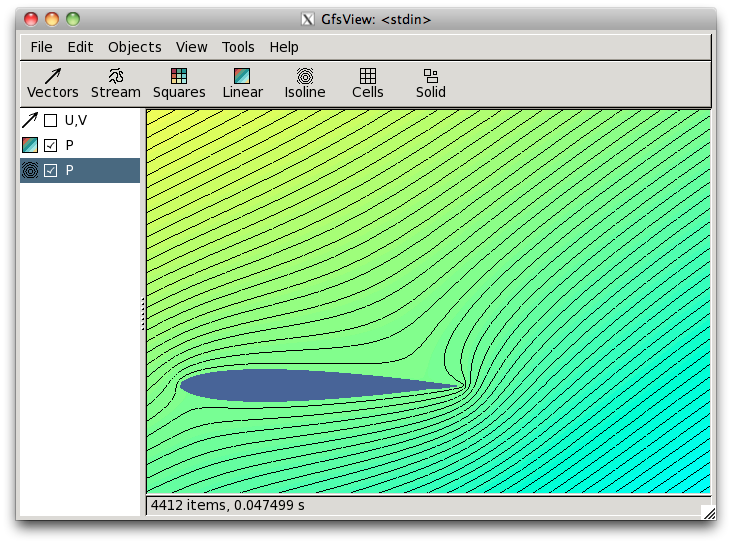
notice that the iso P go round the trailing edge (no Kutta).
Quitting in the menu of gfsview will then allow to compute
the problem with only circulation
(it is the flow in the frame of the wing),
and then
the linear combination to impose the Kutta condition, notice the stream lines at the trailing edge:
run.sh
explores all the angles to plot the circulation (the flat plate is displayed as well)